Fit of Binned Distributions

12. Fit of Binned Distributions#

12.1. Introduction#

The least squares and maximum likelihood methods can also be applied in the case of histograms, i.e., binned distributions, where one wants to fit a function to the distribution of counts in each bin:
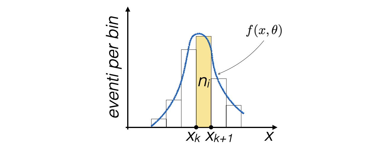
In this case, the content of each bin is a number of events \(n_i\)
If the number of bins and the average number of events in each of them is not small, one can assume that the random variable \(n_i\) follows a Poisson statistic

\[ \mathcal{P}(n,\mu)=\frac{e^{-\mu}\mu^n}{n!} \]

12.1.1. Fit of binned distributions with the least squares method#

In the case of least squares, the function Q²(θ) is usually the following (Neyman’s formulation):

\[ Q^2(\theta) = \sum_{i=1}^N\left(\frac{n_i-f(x_i,\theta)}{\sqrt{n_i}}\right)^2 \]

The value of \(y_i\) from the previous lesson is replaced by \(\mathbf{n_i}\)
The uncertainty on \(\mathbf{n_i}\) is calculated as its square root, as it’s assumed following the Poisson statistic
The value of \(x_i\) is the center of the corresponding bin
The number of bins in the histogram is \(N\)

12.1.2. Fit of binned distributions with the maximum likelihood method#

In the case of maximum likelihood, it is assumed that in each bin the counts follow a Poissonian probability distribution with expected value \(\mu = F_i(\theta)\):

\[ \mathcal{L}(\theta) = \prod_{i=1}^N \frac{e^{-f(x_i,\theta)}F_i(\theta)^{n_i}}{n_i!} \]

where \(F_i(\theta)\) is the expected number of events in each bin

12.1.3. Choosing amongst the least squares and the maximum likelihood#

In the case of few counts present in the bins,
- Bins with zero counts do not contribute to the fit in the case of least squares, despite the absence of events being important information
- It is recommended to use the maximum likelihood method
In the case of many counts present in the bins, the two methods are equivalent, and often the least squares method is computationally simpler

12.2. A regression exercise with binned data#

Starting from a sample of events along a variable x, the objective is to determine the parameters of the probability distribution of the variable
Assuming that this model has a given form, consisting of an exponential background distribution added to a Gaussian signal distribution:

\[\begin{split} \begin{align} f(x) &= N_{B} \cdot \exp(x;\theta_0) + N_{S} \cdot \mathcal{G}(x;\theta_1,\theta_2)\\ &= N_{B} \cdot \frac{1}{\theta_0} e^{-x/\theta_0} + N_{S} \cdot \frac{1}{\sqrt{2\pi}\theta_2}e^{-\frac{1}{2}\left(\frac{x-\theta_1}{\theta_2}\right)^2} \end{align} \end{split}\]

In this model both \(N_{S}\) and \(N_{B}\) are assumed to be unknown, therefore the fit has to be performed with an extended Likelihood

Tip

In the extended likelihood function, the yields of each component are considered as free parameters and a Poisson distribution is assumed

\[\begin{split} \begin{align} \mathcal{L}(\nu,\theta) &= Pois(N; \nu)\mathcal{L}(\theta)\\ &=\frac{\nu^Ne^{-\nu}}{N!}\prod_{i=1}^N \frac{e^{-f(x_i,\theta)}F_i(\theta)^{n_i}}{n_i!}\\ &=\frac{e^{-\nu}}{N!}\prod_{i=1}^N \nu\frac{e^{-f(x_i,\theta)}F_i(\theta)^{n_i}}{n_i!} \end{align} \end{split}\]
Graphically, the model has a decreasing trend that rises when the Gaussian term becomes significant, as shown in the figure:
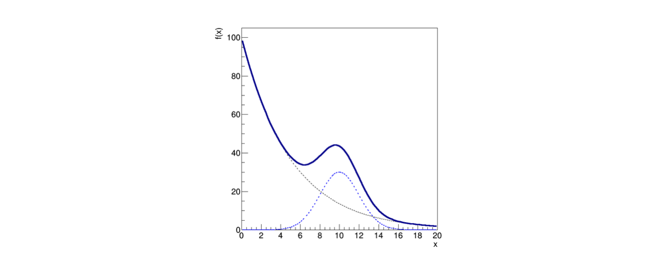
- The solid line represents the total model
- The two dashed lines represent the two terms of the sum, which can be thought of as a signal peak superimposed on a slowly decreasing background

12.2.1. Reading the data from a file#

The starting sample corresponds to a data taking of 10,000 events, stored in the file data.txt
When events are plotted in a histogram, as it’s a counting experiment, the content of each bin fluctuates stochastically:
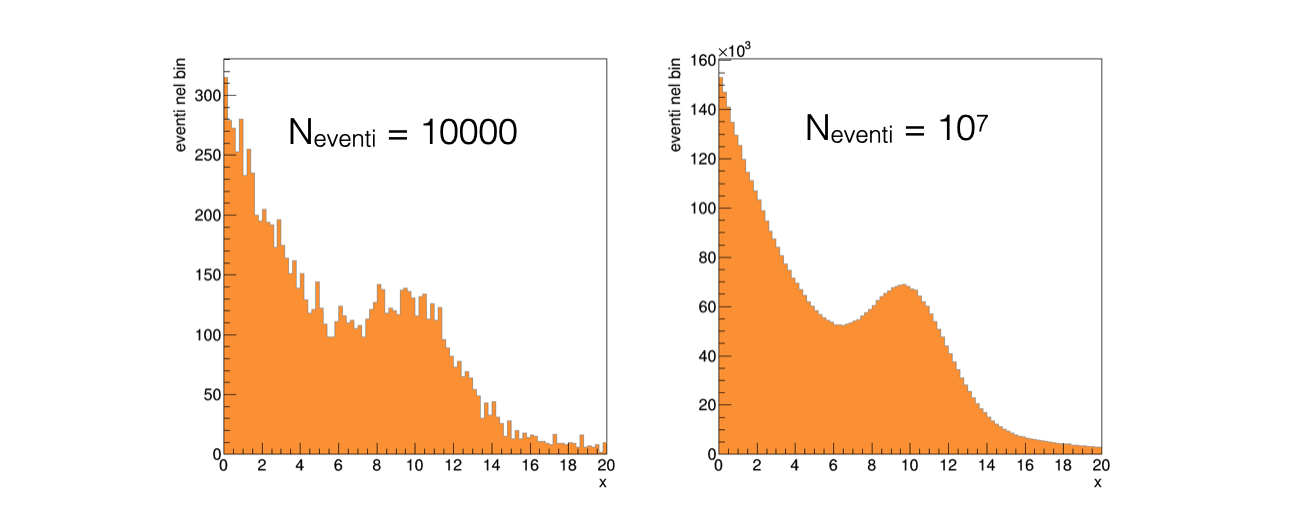
- In the case of 10,000 events, the relative fluctuations are much more visible than in the case of 10,000,000 events, as expected

12.2.2. Determining the fit parameters#

To determine the parameters θ, the extremum of a function needs to be found
- with many parameters
- in the presence of statistical fluctuations
The iminuit library, based on the CERN MINUIT software, offers robust tools to perform this task

12.2.3. Defining the statistical model for the fit#

The minimization performed by the fit is based on the comparison between the number of events observed in each bin with respect to the expectation
This expectation is calculated by integrating the model probability density function

Therefore, the input model iminuit needs to be provided with is based on cumulative distribution functions

def mod_total (bin_edges, N_signal, mu, sigma, N_background, tau):
    return N_signal * norm.cdf (bin_edges, mu, sigma) + \
            N_background * expon.cdf (bin_edges, 0, tau )

The edges of the input histogram are a necessary input for the probability calculations

12.2.4. Setting up the fitting algorithm#

The cost function, for which an extreme has to be found when varying the \(\theta\) parameters, has to be defined (it’s a python object):
```
from iminuit.cost import ExtendedBinnedNLL
# ...
my_cost_func = ExtendedBinnedNLL (bin_content, bin_edges, mod_total)
```

The algorithm that searches for the extreme has to be initialized (it’s also a python object):

my_minuit = Minuit (my_cost_func, 
                    N_signal = N_events, mu = sample_mean, sigma = sample_sigma, # signal input parameters
                    N_background = N_events, tau = 1.)                           # background input parameters

besides the cost function, the algorithm takes as input the initial values of the parameters of mod_total to be used in the search for the extreme

The fit operation is performed with the following command, invoking the least squares method:
```
my_minuit.migrad ()
print (my_minuit.valid)
display (my_minuit)
```
Tip

To load the display function in a python macro
```
from IPython.display import display
```
After the fit, the my_minuit object contains all the information concerning the fit results

12.2.5. Helping Minuit to find the right minimum#

The fit rarely succeeds autonomously as, due to the large number of parameters θ and the stochastic fluctuations of the bin contents, the program struggles to find the correct minimum of the \(Q^2\) function

Some variabiles are bound to be positive:

my_minuit.limits['N_signal', 'N_background', 'sigma', 'tau'] = (0, None)  

To facilitate the fit, it’s very effective to provide the Minuit object with a starting point not far from the final result, based on the knowledge of the problem:
- The parameters N_signal and N_background are the integrals of the two background and signal functions, so they are related to the integral of the histogram:
```
N_events = sum (bin_content)
# and, when initializing the Minuit object:
N_signal = N_events
N_background = N_events
```
- The exponential is certainly decreasing:
```
# when initializing the Minuit object:
tau = 1.
```
- The maximum of the Gaussian is around the middle of the interval (what other options may be chosen to initialize the mu parameter?):
```
sample_mean = np.mean (sample)
# and, when initializing the Minuit object:
mu = sample_mean
```
- The width of the Gaussian is correlated to the histogram sigma for a certain level:
```
sample_sigma = np.std (sample)
# and, when initializing the Minuit object:
sigma = sample_sigma
```

12.2.6. How to deal with one parameter at a time#

Sometimes, even starting from reasonable parameter values, the fit does not converge to the sought extremum
In this case, it can be helpful to identify a region of the x spectrum where only a subset of the parameters is relevant

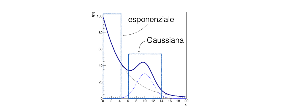
12.2.7. Determine the exponential slope#

A partial fit performed only below \(x = 5\) and above \(x = 15\) with only the parameters of the background component of the model free to float allows to calculate a preliminary estimate of N_background and tau:

# setting the signal to zero for a first background-only preliminary fit
my_minuit.values["N_signal"] = 0
# fixing the value of the signal parameters to a constant value
# (i.e. they are not considered in the fit)
my_minuit.fixed["N_signal", "mu", "sigma"] = True

# temporary mask avoiding the signal region
bin_centres = 0.5 * (bin_edges[1:] + bin_edges[:-1])
my_cost_func.mask = (bin_centres < 5) | (15 < bin_centres)

my_minuit.migrad ()

A second partial fit performed with the background component of the model frozen to the values found so far, which are known to the Minuit object, allows to calculate a preliminary estimate of N_signal, mu and sigma:

my_cost_func.mask = None # remove mask
my_minuit.fixed = False # release all parameters
my_minuit.fixed["N_background", "tau"] = True # fix background parameters
my_minuit.values["N_signal"] = N_events - my_minuit.values["N_background"] # do not start at the limit
my_minuit.migrad ()

12.2.8. The final fit#

For the final fit, all parameters are free to float and the Minuit object will start the extremum search from the result of the last fit performed:
```
my_minuit.fixed = False # release all parameters
my_minuit.migrad ()
print (my_minuit.valid)
display (my_minuit)
```

12.3. Analyzing the regression results#

The result of the fit consists in several pieces of information:
- whether an extremum has been found and how the Minuit algorithm did behave;
- the point value of the parameters at the extreme;
- the uncertainty associated with the result.
The command
```
display (my_minuit)
```
shows the whole information concerning the fit, including a plot of the input data with the fitting model superimposed
Each piece of information may be extracted from the Minuit object, for it to be used in the program

12.3.1. Study the fit convergence#

To determine the success of the numerical algorithm, the Minuit.valid variable is used: which should be True in case of success:
```
print (my_minuit.valid)
```

12.3.2. Parameter values and uncertainty#

As for the least squares case, the value of the parameters and their uncertainty can be obtained from the Minuit object:

for par, val, err in zip (my_minuit.parameters, my_minuit.values, my_minuit.errors) :
    print(f'{par} = {val:.3f} +/- {err:.3f}') # formatted output

The uncertainty is by default calculated by inverting the Hessian matrix of the cost function, which is equivalent to applying the Cramér-Rao theorem assuming that the estimator is unbiased and efficient
To calculate the uncertainty by looking at the likelihood profile, which is a multi-dimensional generalization of the graphic method, an additional call to the minos function needs to be added:
```
my_minuit.minos ()
```

This will produce positive and negative uncertainties which, in general, are not symmetric around each parameter value:

for key in my_minuit.parameters : # parameters is a tuple containing the parameter names
    print ('parameter ' + key + ': ' + 
           str (my_minuit.values[key]) + ' + ' + 
           str (my_minuit.merrors[key].upper) + ' ' + 
           str (my_minuit.merrors[key].lower)
          )

12.4. Unbinned maximum likelihood fit#

In the case of an unbinned maximum likelihood fit, the model function to be used is the probability density function itself. For a Gaussian case:
```
def mod_signal_unb (x, mu, sigma) :
    return norm.pdf(x, mu, sigma)
```

The proper cost function shall be deployed for the fitting:

from iminuit.cost import UnbinnedNLL
# ...
my_cost_func_unb = UnbinnedNLL (subsample, mod_signal_unb)

The fitting functionalities then work in the same way as described for the binned maximum likelihood case
- In this case, the value of the cost function cannot be used as an approximation of the \(Q^2\)

12.5. Least squares and maximum likelihood#

The least squares method (LS) and the maximum likelihood method (ML) are parameter estimators of a model based on data
The two estimators have different properties and exhibit different behaviors: even though they use the same data, they can produce different results

12.5.1. Least squares method for histogram fitting#

When applying the least squares method, the input function representing the statistical model simply scales the probability density function by the total number of events. For a gaussian case:
```
def func_approx (x, N_events, mean, sigma, bin_width) :
    return N_events * norm.pdf (x, mean, sigma) * bin_width
```