Toy Experiments and Integration using Pseudorandom Numbers

8. Toy Experiments and Integration using Pseudorandom Numbers#

8.1. Simulating an experiment with a “Toy Experiment”#

Sequences of pseudo-random numbers are often used to simulate the statistical behavior of a measurement experiment or to perform numerical integrations.
According to the frequentist paradigm of statistics, uncertainties of a measurement are derived from its probability density distribution, assuming that the experiment used for that measurement is repeated a large number of times.
Operationally, the experiment leading to the final measurement result is unique, so certain statistical behaviors can only be simulated.
The simulation of a measurement experiment is called a toy experiment.

8.1.1. Precision on the mean of a sample#

To determine the precision on the mean of a sample, it’s necessary to generate the sample many times to observe the distribution of mean values:
```
from myrand import generate_uniform
# ....
means = []
# loop over toys
for i in range (N_toy):
    randlist = generate_uniform (N_evt)
    toy_stats = stats (randlist)
    means.append (toy_stats.mean ())
```
Note
- The randlist and toy_stats objects is recreated for each toy experiment.
- While the toy_stats object collects the statistics of each individual toy experiment and is used to calculate their mean, the means object collects the sample of mean values for all toy experiments.

8.1.2. Visualizing the distribution of the means#

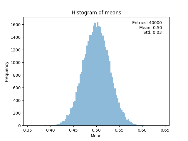
The mean of the measurements is a function of random variables, hence it is a random variable itself.

Its probability distribution is obtained by sampling with toy experiments, by plotting the histogram of the means content:

from stats import stats
# ...
means_stats = stats (means)
xMin = means_stats.mean () - 5. * means_stats.sigma ()
xMax = means_stats.mean () + 5. * means_stats.sigma ()
nBins = floor (len (means) / 10.) + 1     # number of bins of the histogram
bin_edges = np.linspace (xMin, xMax, nBins + 1)  # edges o the histogram bins
fig, ax = plt.subplots ()
ax.set_title ('Histogram of the mean over ' + str (N_toy) + ' toys', size=14)
ax.set_xlabel ('mean value')
ax.set_ylabel ('toys in bin')
ax.hist (means,
         bins = bin_edges,
         color = 'orange',
        )

means

8.1.3. Comparing with the standard deviation of the mean#

The standard deviation of the mean for each individual toy, being the uncertainty associated with the mean of measurements, must correspond to the standard deviation of the sample of means.

To check this correspondence, the stats class can be used:

print ('sigma of the means disitribution:             ', means_stats.sigma ())
print ('mean of the sigma of the means disitribution: ', sigma_means_stats.mean ())

# plot the distribution of the sigma on the mean
# calculated for each toy
xMin = sigma_means_stats.mean () - 5. * sigma_means_stats.sigma ()
xMax = sigma_means_stats.mean () + 5. * sigma_means_stats.sigma ()
nBins = floor (len (sigma_means) / 10.) + 1     # number of bins of the histogram
bin_edges = np.linspace (xMin, xMax, nBins + 1)  # edges o the histogram bins
fig, ax = plt.subplots ()
ax.set_title ('Histogram of the sigma on the mean over ' + str (N_toy) + ' toys', size=14)
ax.set_xlabel ('mean value')
ax.set_ylabel ('toys in bin')
ax.hist (sigma_means,
         bins = bin_edges,
         color = 'orange',
        )

8.2. Integration with pseudo-random numbers#

Sequences of pseudo-random numbers can be effectively used to calculate areas bounded by functions.
Methods that utilize pseudo-random numbers are called Monte Carlo techniques, deriving this name from the famous casino, realm of the goddess of chance.
The use of these techniques in physics is extensive, for example in computing integrals in quantum mechanics and quantum field theory, for simulating measurement apparatuses, and more.

8.2.1. Prerequisites to integrate with pseudo-random numbers#

Let’s consider the case of integrating functions which are positive, continuous, and defined on a compact and connected interval (thus finite over the entire domain).
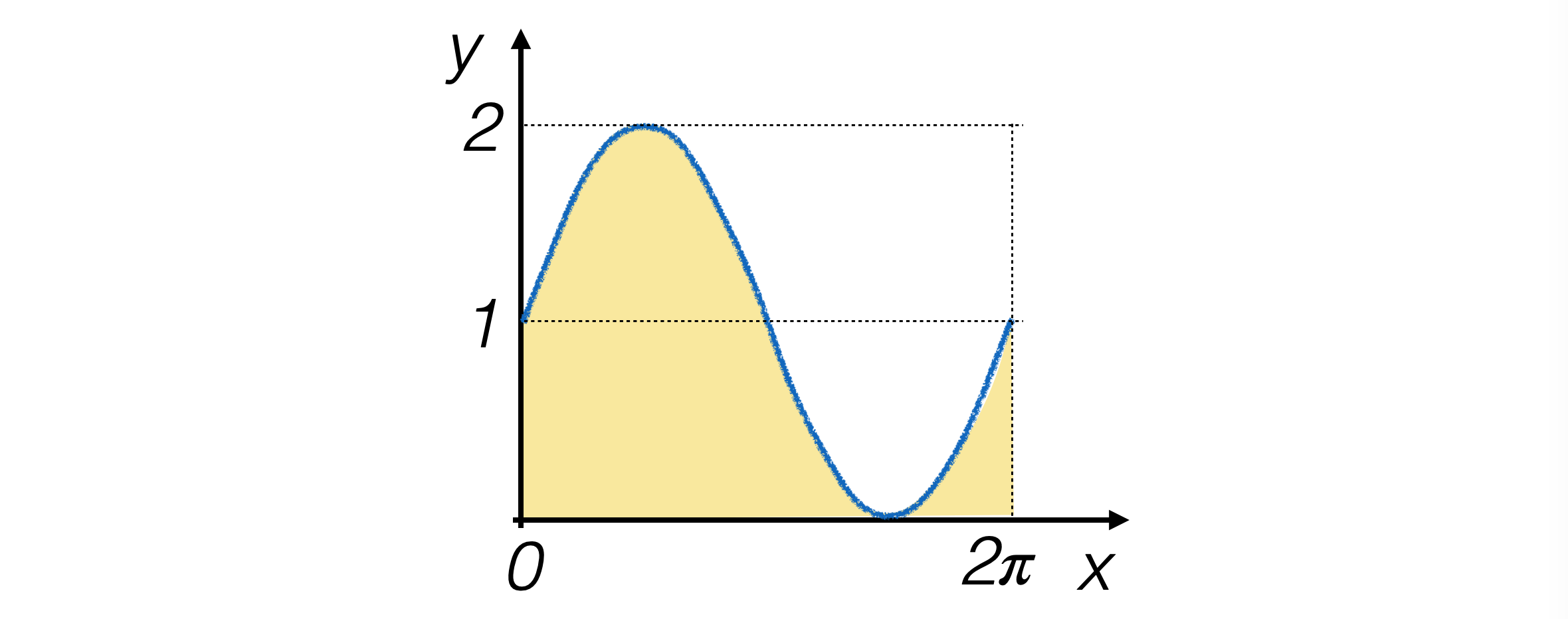
Let’s take the function g(x) = sin(x) + 1 defined on the interval (0, π) as an example.
- For this function, we can analytically calculate the integral, which is 2π.

integral

8.2.2. The hit-or-miss method#

The hit-or-miss algorithm behaves similarly to generating pseudo-random numbers using the try-and-catch technique.
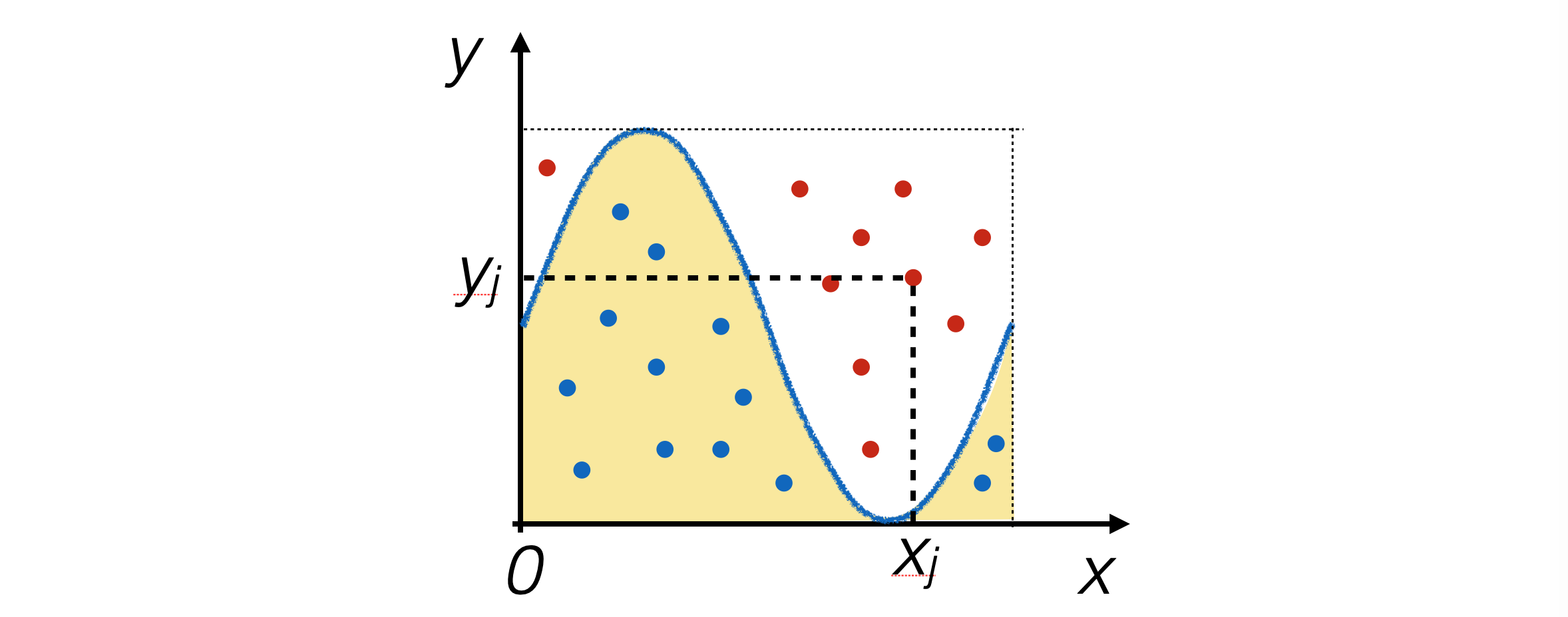
N pairs of pseudo-random numbers are generated in the plane containing the function plot, and the number of events n_hit falling within the area under the function is counted.
Consequently, if A is the area of the rectangle where the events were generated, and m and M are the integration limits:

\[ \underset{N \to \infty}{\lim} \frac{n_{hit}}{N} = \frac{\int_{m}^{M}g(x)dx}{A} \]

8.2.3. Precision of the hit-or-miss method#

Infinite pseudo-random numbers cannot be generated, hence the result will be approximate:

\[ \int_{m}^{M}g(x)dx \simeq A\cdot\frac{n_{hit}}{N}=I \]

The quantity I is the result of the integral for the hit-or-miss method.
Being a function of pseudo-random numbers, it is itself a pseudo-random number.
It has an expected value and a variance.
The latter is the numerical uncertainty in the integral calculation.
- A and N are known without uncertainty.
- n_hit follows a binomial distribution, associating success with a point generated lying below the integrating function, with probability p = n_hit / N.

8.2.4. The numerical uncertainty of the hit-or-miss method#

Expected value and variance of I, given N generated pseudo-random numbers, are therefore:

\[\begin{split} &E[I] = E\left[ A\cdot\frac{n_{hit}}{N} \right] = \frac{A}{N}E[n_{hit}] = \frac{A}{N}\;Np = A\cdot\frac{n_{hit}}{N} \\ &V[I] = V\left[ A\cdot\frac{n_{hit}}{N} \right] = \frac{A^2}{N^2}V[n_{hit}] = \frac{A^2}{N}\;p(1-p) \end{split}\]

Consequently, the numerical uncertainty in the integral calculation is given by the square root of the variance.

8.2.5. The implementation of the hit-or-miss method#

Also in this case, it involves generating pseudo-random numbers on the plane within (0, 2π) on the x axis and (0, 2) on the y axis, and counting how many pairs of points are below the integrating function:

def integral_HOM (func, xMin, xMax, yMax, N_evt) :

    x_coord = generate_range (xMin, xMax, N_evt)
    y_coord = generate_range (0., yMax, N_evt)

    points_under = 0
    for x, y in zip (x_coord, y_coord):
        if (func (x) > y) : points_under = points_under + 1 

    A_rett = (xMax - xMin) * yMax
    frac = float (points_under) / float (N_evt)
    integral = A_rett * frac
    integral_unc = A_rett**2 * frac * (1 - frac) / N_evt
    return integral, integral_unc

Starting from n_hit, then, the integral value and its uncertainty can be calculated.

8.2.6. The crude Monte Carlo method#

The crude Monte Carlo algorithm exploits the properties of the expectation value of a function.
Given a set of pseudo-random numbers x_i generated according to a uniform probability distribution f(x) defined between m and M, the expectation value of the function g(x) turns out to be:

\[ E[g(x)] = \int_{m}^{M}g(x)\;f(x)dx = \int_{m}^{M}g(x)\;\frac{1}{(M-m)}dx = \frac{1}{(M-m)}\int_{m}^{M}g(x)dx \]

by definition of the uniform probability distribution.
E[g(x)] can be estimated using the average of the values g(x_i), and the variance of g(x) can be estimated using the standard deviation of the mean of the values g(x_i), which is calculated from the variance V[g(x)].
Therefore, an estimate of the integral of g(x) and its uncertainty can be calculated:

\[ \int_{m}^{M}g(x)dx = (M-m) \left( E[g(x)] \pm \sqrt{\frac{V[g(x)]}{N}} \right) \]

Note

The examples for the lecture may be found here
The exercises for the lecture may be found here