4. Generation of Pseudo-Random Numbers

4.1. Pseudo-Random Numbers

• When performing any measurements, the comparison between collected data and a model of nature is carried out

  • To falsify the model, or

  • To determine the value (and associated uncertainty) of one of its parameters

• It is therefore crucial to be able to calculate model predictions

  • Often the model is not known in an analytical form and alternative computational methods are used to obtain predictions for comparison with measurements

• Many calculation techniques are based on generating random numbers

  • To reproduce the random nature of measurements

  • Or to uniformly populate phase spaces defined within sophisticated boundaries

4.1.1. Random Sequences

• A random process or stochastic process produces a sequence of numbers randomly distributed according to a fixed probability distribution

• The probability that a particular number appears at any point in the sequence does not depend on the numbers that precede or follow it

• For example:

  • Arrival time of cosmic rays on a muon detector

  • The result of a coin toss or dice roll

• Since they depend on the timing of natural processes, these are typically sequences that take a long time to construct, which becomes a limiting factor in calculations

4.1.2. Pseudo-Random Sequences

• Programs and libraries exist, generally called pseudo-random number generators, that produce sequences of numbers that appear random

• The sequence of numbers in these sequences is deterministic, and the functions used for generation are designed to mimic the behavior of random sequences

• The first number in a sequence of pseudo-random numbers is called the seed, because that number is known and, along with the generation algorithm, the entire sequence can be reproduced

  • Different seeds will start different sequences of pseudo-random numbers, or start the same sequence from different points

4.1.3. Linear Congruential Generator

• An example of a formula to calculate the next element of a pseudo-random sequence given any number is as follows:

  \[ x_{n+1} = (A \cdot x_n + C) \mod M \]

• With:

  \[\begin{split} M &> 0 \\ 0 <~&A < M \\ 0 <~&x_0 < M \\ M &\sim 10^{32} \end{split}\]

• The first element of the sequence, with index zero, is the seed

• This algorithm generates by construction numbers between 0 and M

4.1.4. Issues with Pseudo-Random Number Generators

• The functional dependence between two consecutive pseudo-random numbers should not be visible in the samples used for data analysis

• If a repeated number reappears in a pseudo-random sequence, the sequence starts repeating from that point: this is the periodicity of the generator

• The period must be much greater than the quantity of generated pseudo-random numbers and should not depend on the seed choice

• Typically, random number generators follow a uniform distribution: non-uniformity of the distribution is another common defect that one wants to avoid

• An example of the result of a poorly performing pseudo-random number generator can be found here

4.1.5. A Random Number Generator in Python

• The random library contains a pseudo-random number generator random():

  import random
  
  randlistint = [] 
  for i in range (5):
      # Return the next random floating point number in the range 0.0 <= X < 1.0
      randlist.append (random.random ())
      print (i, randlist[-1])
  

  The code above produces the following output:

  0 0.9773950056543294
  1 0.6500404225224424
  2 0.042647579579998096
  3 0.8110944794319123
  4 0.6975819042310242
  

4.1.6. Characteristics of random

• It is a generator of pseudo-random numbers uniformly distributed between 0 and 1

• The default seed of the random function is set based on the current time as known by the operating system

• To have the generator starting from a given seed, so that the same sequence is produced ad every run of the script, the following instruction has to be used:

  random.seed ( seed ) # seed can be any floating point number
  

• It’s in fact important to be able to reproduce the same sequence of pseudo-random numbers for testing purposes.

• Unless there are important reasons to do otherwise, the seed is initialized only once during the execution of a program.

4.1.7. Generating integer random-numbers

• The random library may be used to generate integer numbers as well:

  randlistint = []
  for i in range (5):
      # Return the next random floating point number in the range 0.0 <= X < 1.0
      randlistint.append (random.randint (0, 100))
      print (i, randlistint[-1])
  

  • The randint function generates numbers within a range specified in its arguments

4.2. Generating Pseudo-Random Numbers with Uniform Distribution

• The random library may be used to produce sequences of pseudo-random numbers following different distributions using appropriate algorithms.

• Usually, the probability density functions of pseudo-random numbers generated with a computer will have a limited range, due to intrinsic limitations of computers.

• The uniform distribution of random numbers is a special case, as it is defined on a limited set by construction (otherwise its integral would be divergent).

4.2.1. Uniform Distribution of Pseudo-Random Rational Numbers

• The goal is to produce random numbers within the interval min, max, using the resources at hand, i.e., random.

  1. Uniform distribution between 0 and 1:

     random.random ()
     

  2. Scaling between 0 and max-min:

     (max - min) * random.random () 
     

  3. Translation by min:

     def rand_range (xMin, xMax) :
         '''
         generazione di un numero pseudo-casuale distribuito fra xMin ed xMax
         '''
         return xMin + random.random () * (xMax - xMin)
     

4.3. Other Probability Distributions: Try-and-Catch

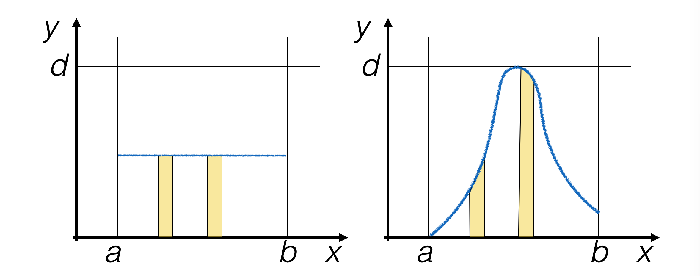
• In the case of the uniform probability density function (PDF), the probability that pseudo-random events are generated in a given interval does not depend on the position of the interval.

• For non-uniform PDFs, this is not true.

4.3.1. The Try-and-Catch (TAC) Algorithm

• Generate pseudo-random events in a way proportional to the area under the PDF.

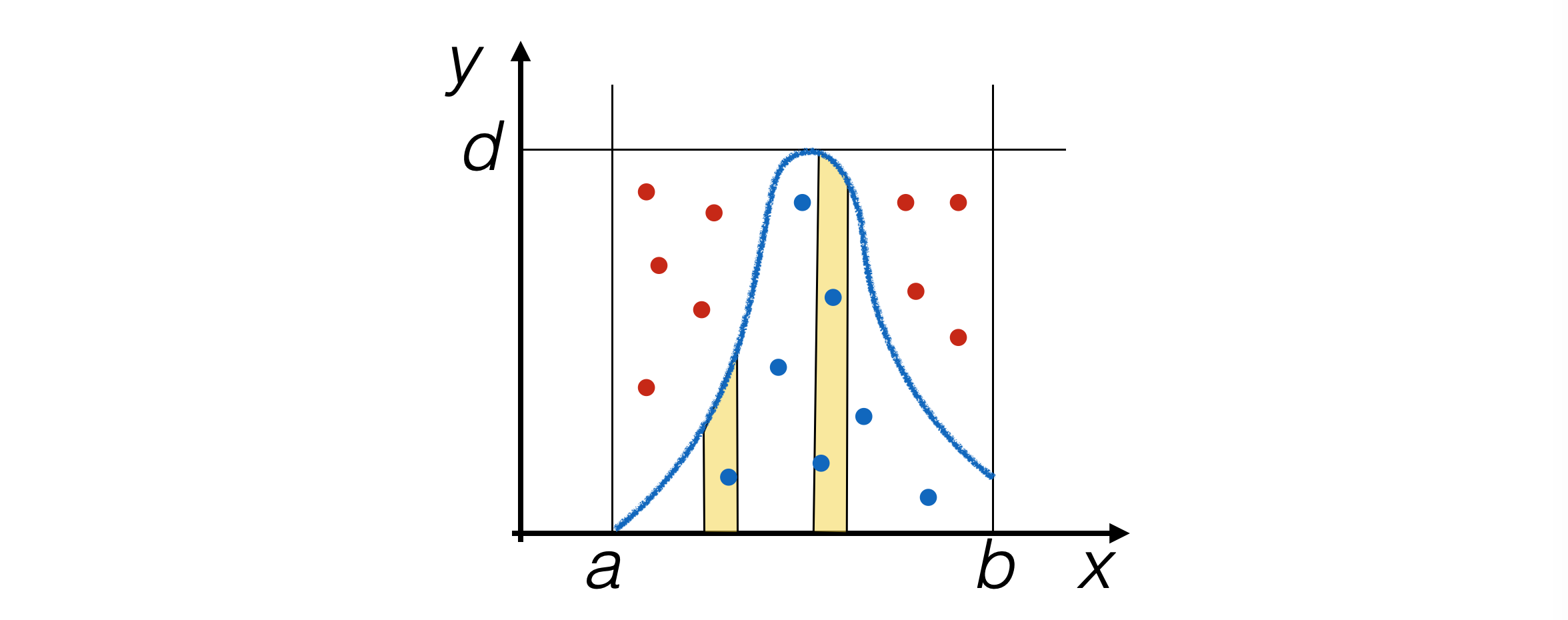
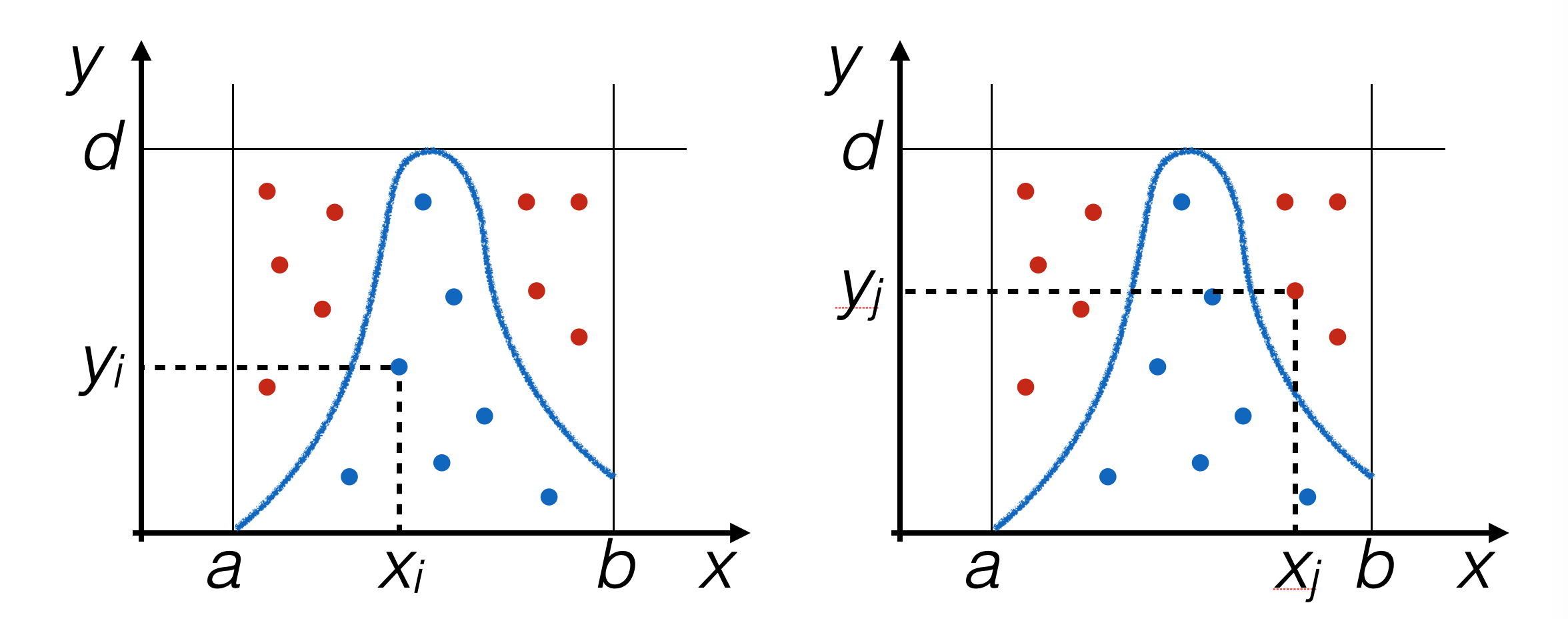
• Populate the plane with pairs of pseudo-random numbers x,y, each generated uniformly with rand_range (), and use x only if y < f(x).

4.3.2. Implementation of the Try-and-Catch Algorithm

• To repeat generation until the condition y < f(x) is satisfied, a loop is used:

  def rand_TAC (f, xMin, xMax, yMax) :
      '''
      generazione di un numero pseudo-casuale 
      con il metodo try and catch
      '''
      x = rand_range (xMin, xMax)
      y = rand_range (0, yMax)
      while (y > f (x)) :
          x = rand_range (xMin, xMax)
          y = rand_range (0, yMax)
      return x
  

• The function rand_TAC needs more arguments than rand_range:

  • an upper limit for the vertical axis: yMax

  • the functional form to be used as the PDF: as you can see, a function can also be passed as an argument to another function simply by name.

Important

Advantages

• Knowing the functional form of the PDF, the algorithm works.

• It’s not necessary for the PDF to be known analytically, as it’s sufficient that it can be written as a python function.

• Easily generalizable to N dimensions.

Disadvantages

• One must be sure to know the maximum (yMax) of the function.

• It has low efficiency:

  • To obtain a random number, at least two are generated.

  • Often many more, because many points on the plane are discarded.

4.4. Other Probability Distributions: Inverse Function

• Let x be a random variable with continuous PDF f(x).

• Let F(x) be its cumulative distribution function (CDF).

• If F(x) is strictly increasing, then the variable y = F(x) has a uniform distribution. (This is proved using the chain rule when changing variables in a PDF.)

• Generating pseudo-random events with uniform distribution in y is therefore equivalent to generating pseudo-random events along x with distribution f(x).

4.4.1. The Inverse Function Algorithm

• Calculate analytically F(x) and its inverse function F ^-1(y).

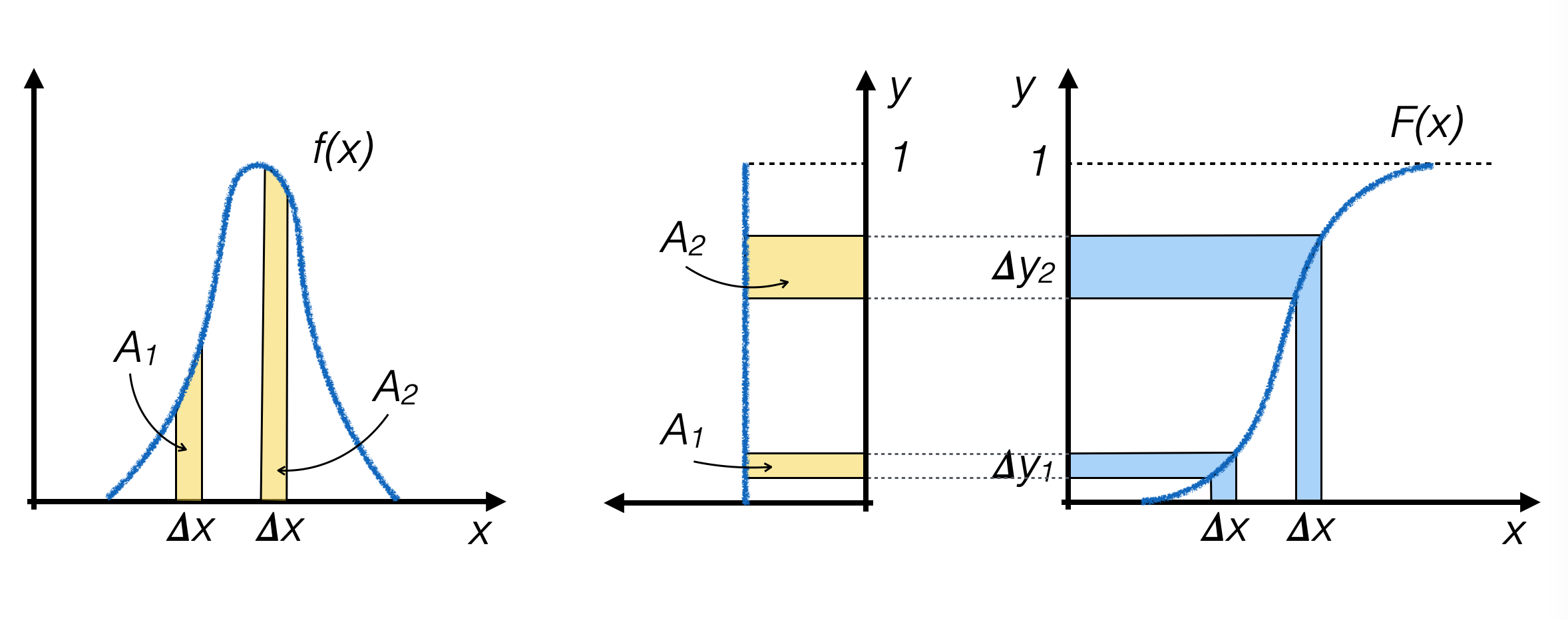
• Generate pseudo-random numbers y_i with uniform distribution between 0 and 1 along the y axis.

• For each generated event, calculate x_i = F ^-1(y_i) and use that value as the generated random number.

• Where f(x) is higher, F(x) is steeper, so the number of pseudo-random numbers generated in the two intervals Δy₁ and Δy₂ is proportional to the area under the curve f(x) above the two intervals with width Δx, respectively, which is the goal to achieve.

Important

Advantages

• It’s efficient in generating pseudo-random numbers, as each number is used.

Disadvantages

• One must know the analytical form of f(x) and F(x) and be able to invert the cumulative function to obtain F ^-1(y).

• Calculating a function adds time to the event generation.

4.5. Gaussian Probability Distributions: Central Limit Theorem

• The central limit theorem can be used to generate probability distributions with Gaussian shape.

  The central limit theorem

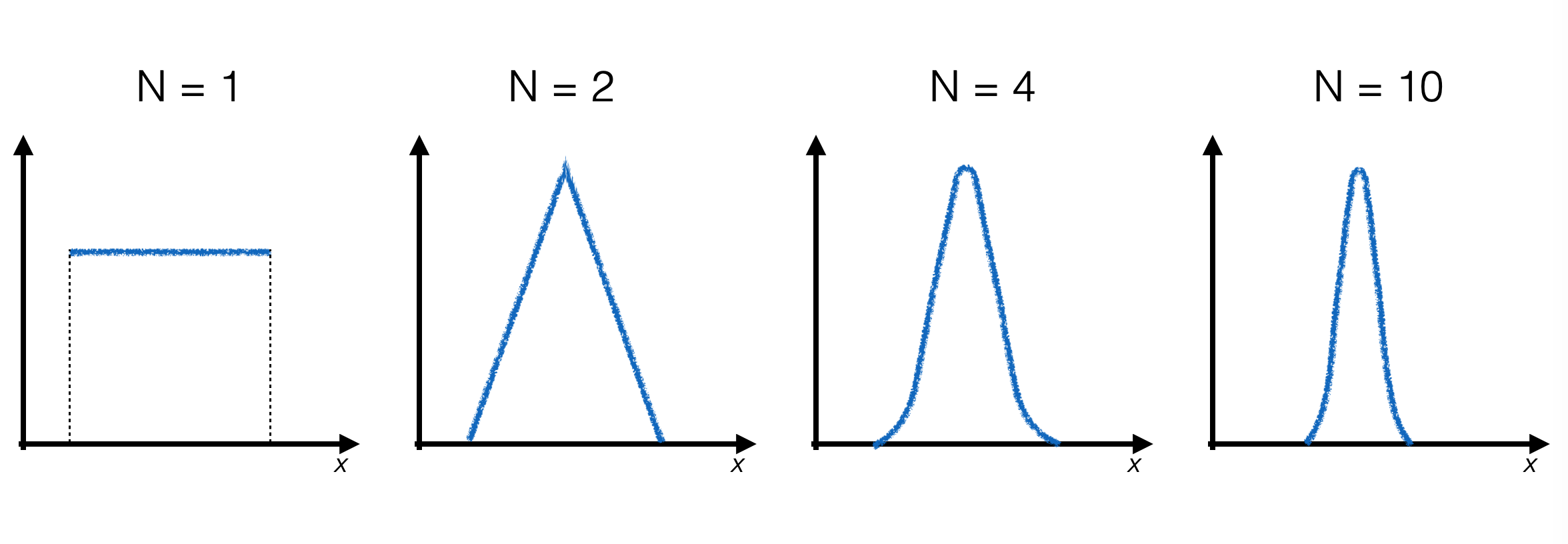
  Let N be given independent and identically distributed random variables x_i with probability distribution f(x) having finite mean μ and variance σ². Then, for large N, the variable y = ⟨x_i⟩ is distributed as a Gaussian with mean μ and variance σ²/N.

4.5.1. Implementation of the Algorithm

• In this case as well, we start with a known pseudo-random number generator - the uniform distribution.

• To produce a single pseudo-random number distributed according to a Gaussian, it’s necessary to generate N pseudo-random numbers according to the uniform distribution and calculate their average.

• As N increases, the final distribution gets closer and closer to the Gaussian limit:

Important

Advantages

• It’s based on a well-known theorem and allows for (within the numerical approximations of a computer) verification that the theorem works.

• It’s not necessary to analytically describe the functional form of the Gaussian.

Disadvantages

• To achieve good precision, many uniform pseudo-random numbers need to be generated to obtain one distributed according to a Gaussian distribution.

Note

• The examples for the lecture may be found here

• The exercises for the lecture may be found here