11.6. Least squares solutions#
11.6.1. Exercise 11.1#
After defining, in a dedicated library, a linear function \(\phi(x, \theta)\) with two parameters \(\theta\):
Write a program that generates a set of 10 pairs \((x_i, y_i)\) such that the points \(x_i\) are randomly distributed along the horizontal axis between 0 and 10, and the points \(y_i\) are constructed using the formula \(y_i = \phi(x_i, \theta) + \epsilon_i\).
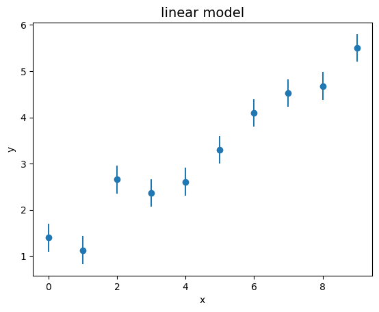
Plot the obtained sample, including the expected error bars.
# the model to be used for the exercise

def func (x, m, q) :
    '''
    reference model to be fitted
    '''
    return m * x + q

# initial parameters of the problem

m_true = 0.5
q_true = 1.1
epsilon_sigma = 0.3
from matplotlib import pyplot as plt
import numpy as np
from myrand import generate_TCL_ms

epsilons = generate_TCL_ms (0., epsilon_sigma, 10)

x_coord = np.arange (0, 10, 1)
y_coord = np.zeros (10)
for i in range (x_coord.size) :
    y_coord[i] = func (x_coord[i], m_true, q_true) + epsilons[i]

sigma_y = epsilon_sigma * np.ones (len (y_coord))

fig, ax = plt.subplots ()
ax.set_title ('linear model', size=14)
ax.set_xlabel ('x')
ax.set_ylabel ('y')
ax.errorbar (x_coord, y_coord, xerr = 0.0, yerr = sigma_y, linestyle = 'None', marker = 'o')
plt.show ()

11.6.2. Exercise 11.2#
Use the iMinuit library to perform a fit on the simulated sample.
Check if the fit was successful.
Print the values of the determined parameters and their sigmas on the screen.
from iminuit import Minuit
from iminuit.cost import LeastSquares

# generate a least-squares cost function
least_squares = LeastSquares (x_coord, y_coord, sigma_y, func)
my_minuit = Minuit (least_squares, m = 0, q = 0)  # starting values for m and q
my_minuit.migrad ()  # finds minimum of least_squares function
my_minuit.hesse ()   # accurately computes uncertainties
# NB: adding additional instructions prevents the automatic visualisation of the fit result
| Migrad | |
|---|---|
| FCN = 10.67 (χ²/ndof = 1.3) | Nfcn = 40 |
| EDM = 2.69e-21 (Goal: 0.0002) | |
| Valid Minimum | Below EDM threshold (goal x 10) |
| No parameters at limit | Below call limit |
| Hesse ok | Covariance accurate |
| Name | Value | Hesse Error | Minos Error- | Minos Error+ | Limit- | Limit+ | Fixed | |
|---|---|---|---|---|---|---|---|---|
| 0 | m | 0.467 | 0.033 | |||||
| 1 | q | 1.12 | 0.18 |
| m | q | |
|---|---|---|
| m | 0.00109 | -0.0049 (-0.843) |
| q | -0.0049 (-0.843) | 0.0311 |
# information about the function minimum can be directly accessed with Minuit.fmin
my_minuit.fmin
| Migrad | |
|---|---|
| FCN = 10.67 (χ²/ndof = 1.3) | Nfcn = 40 |
| EDM = 2.69e-21 (Goal: 0.0002) | |
| Valid Minimum | Below EDM threshold (goal x 10) |
| No parameters at limit | Below call limit |
| Hesse ok | Covariance accurate |
# global characteristics of the fit
is_valid = my_minuit.valid
print ('success of the fit: ', is_valid)
success of the fit: True
# fit parameters
for par, val, err in zip (my_minuit.parameters, my_minuit.values, my_minuit.errors) :
    print(f'{par} = {val:.3f} +/- {err:.3f}') # formatted output

m_fit = my_minuit.values[0]
q_fit = my_minuit.values[1]
m = 0.467 +/- 0.033
q = 1.125 +/- 0.176
11.6.3. Exercise 11.3#
Calculate the value of \(Q^2\) using the points and the fitted function obtained in the previous exercise.
Compare the value obtained with
iminuitwith the calculated one.Print the value of the degrees of freedom of the fit
Q_squared = my_minuit.fval
print ('value of the fit Q-squared', Q_squared)
N_dof = my_minuit.ndof
print ('value of the number of degrees of freedom', N_dof)
value of the fit Q-squared 10.66504489575817
value of the number of degrees of freedom 8.0
Q_squared_calc = 0.
for x, y, ey in zip (x_coord, y_coord, sigma_y) :
    Q_squared_calc = Q_squared_calc + pow ( (y - func (x, m_fit, q_fit)) /ey , 2 )
print ('Difference between Q-squared values:', Q_squared_calc - Q_squared)
Difference between Q-squared values: -1.7763568394002505e-15
11.6.4. Exercise 11.4#
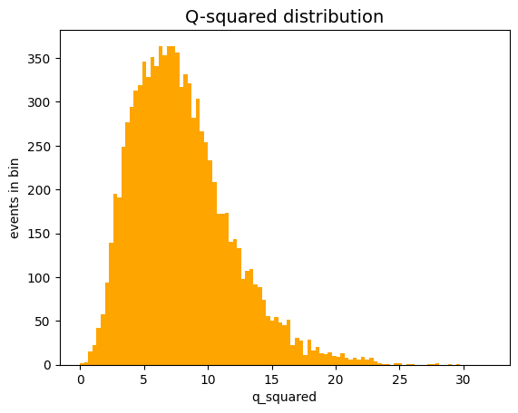
Using the toy experiments technique, generate 10,000 fit experiments with the model studied in the previous exercises and fill a histogram with the obtained values of \(Q^2\).
Compare the expected value of \(Q^2\) obtained from the toy experiments with the degrees of freedom of the problem.
from math import floor
from stats import stats

N_toys = 10000
Q_squares = []
x_coord_toy = np.arange (0, 10, 1)
y_coord_toy = np.zeros (10)

for i_toy in range (N_toys) :
    epsilons_toy = generate_TCL_ms (0., epsilon_sigma, 10)
    for i in range (x_coord_toy.size) :
        y_coord_toy[i] = func (x_coord_toy[i], m_true, q_true) + epsilons_toy[i]
    least_squares = LeastSquares (x_coord_toy, y_coord_toy, sigma_y, func)
    my_minuit_toy = Minuit (least_squares, m = 0, q = 0)  # starting values for m and q
    my_minuit_toy.migrad ()  # finds minimum of least_squares function
    my_minuit_toy.hesse ()   # accurately computes uncertainties
    if my_minuit_toy.valid :
        Q_squares.append (my_minuit_toy.fval)

fig, ax = plt.subplots ()
ax.set_title ('Q-squared distribution', size=14)
ax.set_xlabel('q_squared')
ax.set_ylabel('events in bin')
bin_edges = np.linspace (0, 4 * N_dof, floor (N_toys/100))   # edges o the histogram bins
ax.hist (Q_squares,
         bins = bin_edges,
         color = 'orange',
        )
plt.show ()

Q_squares_stats = stats (Q_squares)
print ('average Q_squared expected value:', Q_squares_stats.mean ())

average Q_squared expected value: 7.968485056644232
11.6.5. Exercise 11.5#
Modify the previous program by deliberately changing the experimental uncertainty associated with the points \(y_i\) in the sample and verify that it’s possible to recover the uncertainty used in generating the points through the expected value of the variable \(Q^2\).
from math import floor, sqrt
from stats import stats

N_toys = 10000
Q_squares_mod = []
x_coord_toy = np.arange (0, 10, 1)
y_coord_toy = np.zeros (10)
epsilon_sigma_mod = 0.4 * epsilon_sigma

for i_toy in range (N_toys) :
    epsilons_toy = generate_TCL_ms (0., epsilon_sigma_mod, 10)
    for i in range (x_coord_toy.size) :
        y_coord_toy[i] = func (x_coord_toy[i], m_true, q_true) + epsilons_toy[i]
    least_squares = LeastSquares (x_coord_toy, y_coord_toy, sigma_y, func)
    my_minuit_toy = Minuit (least_squares, m = 0, q = 0)  # starting values for m and q
    my_minuit_toy.migrad ()  # finds minimum of least_squares function
    my_minuit_toy.hesse ()   # accurately computes uncertainties
    if my_minuit_toy.valid :
        Q_squares_mod.append (my_minuit_toy.fval)

Q_squares_mod_stats = stats (Q_squares_mod)
print ('average Q_squared expected value:', Q_squares_mod_stats.mean ())
print ('sigma scale factor:', sqrt (Q_squares_mod_stats.mean () / N_dof))
print ('sigma:', epsilon_sigma_mod / sqrt (Q_squares_mod_stats.mean () / N_dof))
average Q_squared expected value: 1.282655199900555
sigma scale factor: 0.40041466005575943
sigma: 0.29968932701737117
11.6.6. Exercise 11.6#
Add to Exercise 11.3 the screen printout of the entire covariance matrix of the fit parameters.
print (my_minuit.covariance)
┌───┬─────────────────┐
│   │       m       q │
├───┼─────────────────┤
│ m │ 0.00109 -0.0049 │
│ q │ -0.0049  0.0311 │
└───┴─────────────────┘
print ('variance of the first parameter (m):', my_minuit.covariance[0][0])
print ('variance of the second parameter (q):', my_minuit.covariance[1][1])
print ('covariance of the two parameters:', my_minuit.covariance[1][0])
variance of the first parameter (m): 0.0010909088206825265
variance of the second parameter (q): 0.03109090126527661
covariance of the two parameters: -0.004909089438271051
11.6.7. Exercise 11.7#
Repeat the fitting exercise for a parabolic trend.
def para (x, a, b, c) :
    '''
    reference model to be fitted
    '''
    return a + b * x + c * x * x

# initial parameters of the problem

a_true = -1.
b_true = 0.7
c_true = 0.3

epsilon_sigma = 1.5
epsilons = generate_TCL_ms (0., epsilon_sigma, 10)

x_coord = np.arange (0, 10, 1)
y_coord = np.zeros (10)
for i in range (x_coord.size) :
    y_coord[i] = para (x_coord[i], a_true, b_true, c_true) + epsilons[i]

sigma_y = epsilon_sigma * np.ones (len (y_coord))

least_squares = LeastSquares (x_coord, y_coord, sigma_y, para)
my_minuit = Minuit (least_squares, a = 0., b = 0., c = 0.)
my_minuit.migrad ()  # finds minimum of least_squares function
my_minuit.hesse ()   # accurately computes uncertainties
| Migrad | |
|---|---|
| FCN = 6.668 (χ²/ndof = 1.0) | Nfcn = 70 |
| EDM = 1.78e-19 (Goal: 0.0002) | |
| Valid Minimum | Below EDM threshold (goal x 10) |
| No parameters at limit | Below call limit |
| Hesse ok | Covariance accurate |
| Name | Value | Hesse Error | Minos Error- | Minos Error+ | Limit- | Limit+ | Fixed | |
|---|---|---|---|---|---|---|---|---|
| 0 | a | -1.9 | 1.2 | |||||
| 1 | b | 1.2 | 0.6 | |||||
| 2 | c | 0.26 | 0.07 |
| a | b | c | |
|---|---|---|---|
| a | 1.39 | -0.6 (-0.810) | 0.051 (0.664) |
| b | -0.6 (-0.810) | 0.372 | -0.038 (-0.963) |
| c | 0.051 (0.664) | -0.038 (-0.963) | 0.00426 |
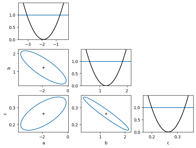
# show the likelihood scans for the various parameters in 1D and 2D
my_minuit.draw_mnmatrix()
(<Figure size 640x480 with 9 Axes>,
 array([[<Axes: >, <Axes: >, <Axes: >],
        [<Axes: ylabel='b'>, <Axes: >, <Axes: >],
        [<Axes: xlabel='a', ylabel='c'>, <Axes: xlabel='b'>,
         <Axes: xlabel='c'>]], dtype=object))

